11 APPENDIX S1

11.1 The PhenoCam network, data processing and selection

The PhenoCam network (https://phenocam.sr.unh.edu) uses digital camera imagery to monitor ecosystem dynamics over time. The network currently consists of over 400 cameras in the conterminous US, tracking vegetation development. Camera imagery is uploaded and stored on the PhenoCam server. Any new images that have been uploaded to the server during the previous 24 hours are converted into greenness time series from RGB triplets of the recorded JPEG images.

Variability in RGB triplets, due to changing scene illumination, can be largely suppressed by converting the DN triplets to their respective chromatic coordinates (e.g. the green chromatic coordinate, Gcc) and subsequent selection of the 90th percentile of the values across a 1 or 3-day period (Richardson et al. 2007, 2009; Sonnentag et al. 2012). Numerous studies have demonstrated the value of the Gcc index (and the corresponding red chromatic coordinate, Rcc) for characterizing the seasonal trajectory of vegetation color and activity (Keenan et al. 2014; Klosterman et al. 2014; Toomey et al. 2015). Furthermore an appropriate “region of interest” (ROI) is defined, corresponding to the area within each digital image for which colour information will be extracted according to the dominant vegetation type in each image. We therefore calculated Gcc as in eq. 1, where X DN denotes the mean (across the ROI) digital number for colour channel X. The generation of these PhenoCam Gcc 1- or 3-day summary product time series is done nightly on the PhenoCam servers.

Gcc = green DN / (red DN + green DN + blue DN) [eq.1]

11.2 The phenocamr R package: methodology

11.2.1 Outlier detection and smoothing

A first step in the post-processing of the PhenoCam data after downloading the data is the detection of outliers which might confound further analysis. For the outlier detection we rely on an iterative spline-based outlier detection algorithm on each of the GCC time series (mean, 50th, 75th, and 90th quantiles) included in the 1- and 3-day summary product files. First, using a range of smoothing factors, we fit a family of cubic smoothing splines to each of time series. We selected the optimal spline from within this family using Akaike’s Information Criterion (AIC, (Akaike 1974)), which balances goodness-of-fit against model complexity in order to avoid over-fitting (Hurvich et al. 1998). Then, in an iterative process, we identified and flagged data points lying more than 2x standard deviations (based on the residual variance,) from the spline. With these outliers excluded, we then repeated the spline fitting process. This was done up to 20 times or until no further outliers were detected from one iteration to the next. The spline fitting process is repeated one final time, so that together with the outlier flags, a smoothed and interpolated time series (with uncertainty estimates) could be used for transition date estimation. The procedure described above can be applied to either 1- or 3-day summary file using both the detect_outliers() and smooth_ts() routines separately. However, it is preferred to specify the proper post-processing routines upon downloading the PhenoCam data using the download_phenocam() function.

11.2.2 Phenophase estimation

Changes in the cycle of vegetation activity are identified as change points using the Pruned Exact Linear Time (PELT) method (Killick et al. 2011) for each cycle with a penalty factor (beta = 0.5) and a minimum segment length of 14 days. Extracted phenophases are calculated as changes in the signal between these change points and intended to define the start of the “greenness rising” and end of the “greenness falling” stage for a full cycle of vegetation activity (i.e., from dormancy, through green-up or “greenness rising”, peak activity, senescence or “greenness falling”, and back to dormancy). Thus, unlike sigmoid-based approaches that have been typically used in the literature (Zhang et al. 2003; Hufkens et al. 2012; Klosterman et al. 2014; Filippa et al. 2016), our method is not limited to ecosystems with a single annual cycle of green-up and senescence and invariant to changes in baseline values due to varying camera settings over time (see Figure 11.1).

The AIC-selected smoothing spline, described in the previous section, is central to this method. The spline is first used to determine the GCC minima (the baseline before a “greenness rising” stage or after a “greenness falling” stage) and maxima (the peak between “rising” and “falling” stages). From the GCC minima and maxima associated with each stage, we then used the spline to identify the dates when 10%, 25%, and 50% of the amplitude (= maxima – minima) were reached. Different threshold values may be specified by calling the underlying function transition_dates(). Transition date uncertainties were then derived from the confidence interval (1.96 x SE) around the smoothing spline, with a minimum uncertainty extending to the immediately preceding or following observation (i.e., ± 1 and ± 3d for the 1- and 3-day GCC time series, respectively; larger in the case of missing data on either side of the estimated transition date). By default all dates are reported in unix time with a start date at (1970-01-01).

11.3 The phenocamr R package: usage

The phenocamr package, most prominently, interfaces with the PhenoCam server to facilitate easy downloading of pre-processed Gcc time series (see section 2) into the R environment. Subsequently, the package screens for outliers in the downloaded time series, smooths the time series and finally estimates different phenophases in a seamless routine. The phenocamr package currently provides all post-processing of PhenoCam standardized datasets (e.g. V1.0; Richardson et al. 2017, in press). The download_phenocam() function in the package covers most of this functionality. An example of the basic function is provided here:

download_phenocam(site = “bartlett”,
                    vegetation = “DB”,
                    roi_id = 0003,
                    frequency = 3,
                    outlier_detection = TRUE,
                    smooth = TRUE,
                    phenophase = TRUE)

These instruction download 3-day summary data (frequency = 3) at the Bartlett experimental forest site (site = “bartlett”) for a deciduous broadleaf (DB) ROI (vegetation = “DB”) with ID 0003 (roi_id = 0003). In addition, we specify that outlier detection and smoothing should be applied (outlier_detection, and smooth set to TRUE). Finally, phenophases are estimated for this particular time series (phenophase = TRUE). By default transition dates for the 10, 25 and 50% amplitude threshold are estimated for both rising and falling parts of a Gcc time series. A processed Gcc time series at a 3-day time step together with the 25% amplitude of the rising falling stages of each cycle of vegetation activity at the Bartlett experimental forest are shown in 11.1. In the interest of brevity we refer to the package documentation for additional parameter options.

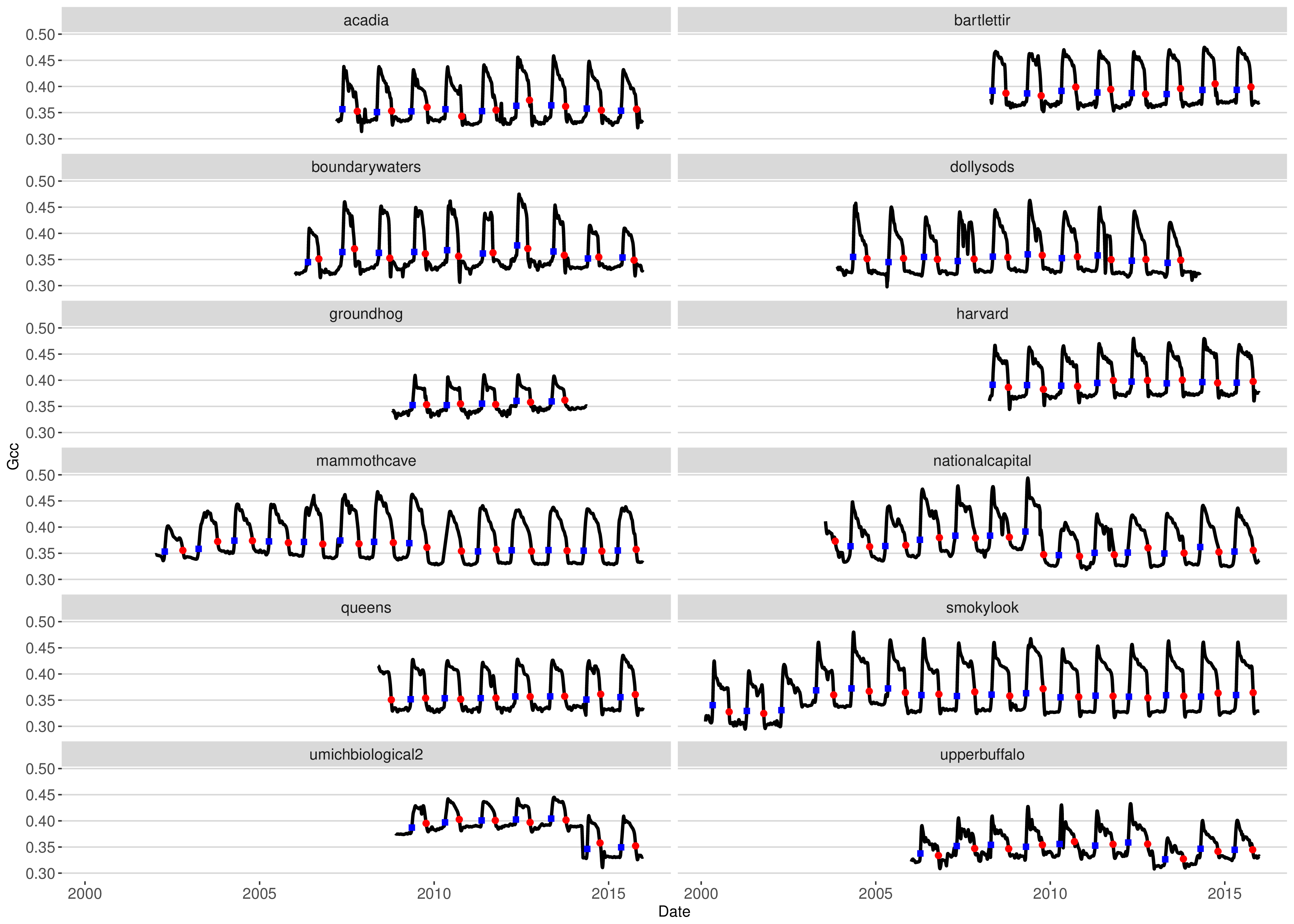
Figure 11.1: Example Gcc PhenoCam Dataset V1.0 time series

11.4 The daymetr R package

Daymet provides gridded estimates of daily weather parameters across North America (Thornton et al. 1997), and makes these data available through an ORNL DAAC web service, to which the daymetr R package provides an interface. A simple download command for a particular location can be executed using the following syntax:

download_daymet( site = "bartlett",
                        lat = 44.0646,
                lon = -71.2881,
                        start = 1980,
                    end = 2010,
                        internal = TRUE)

Here we specify the filename to assign to the data to be downloaded (e.g. “bartlett”) as specified by a given latitude and longitude and a start and end year (start = 1980 and end = 2010, respectively). The ‘internal’ parameter specifies if data should be loaded into the current R workspace (TRUE) or merely downloaded as a comma delimited file (CSV, FALSE) to disk. A similar syntax is used for batch downloading data from a list of locations stored in a CSV file using download_daymet_batch() or downloading gridded (spatial) data through the download_daymet_tiles() and download_daymet_ncss() functions.

11.5 References

Akaike, H. (1974). A new look at the statistical model identification. Automatic Control, IEEE Transactions on, 19, 716–723.

Filippa, G., Cremonese, E., Migliavacca, M., Galvagno, M., Forkel, M., Wingate, L., Tomelleri, E., Morra di Cella, U. & Richardson, A.D. (2016). Phenopix: A R package for image-based vegetation phenology. Agricultural and Forest Meteorology, 220, 141–150.

Hufkens, K., Friedl, M., Sonnentag, O., Braswell, B.H., Milliman, T. & Richardson, A.D. (2012). Linking near-surface and satellite remote sensing measurements of deciduous broadleaf forest phenology. Remote Sensing of Environment, 117, 307–321.

Hurvich, C.M., Simonoff, J.S. & Tsai, C.-L. (1998). Smoothing parameter selection in nonparametric regression using an improved Akaike information criterion. Journal of the Royal Statistical Society: Series B (Statistical Methodology), 60, 271–293.

Keenan, T., Darby, B., Felts, E., Sonnentag, O., Friedl, M., Hufkens, K., O’Keefe, J., Munger, J.W., Toomey, M. & Richardson, A.D. (2014). Tracking forest phenology and seasonal physiology using digital repeat photography: a critical assessment. Ecological Applications.

Killick, R., Fearnhead, P. & Eckley, I.A. (2011). Optimal detection of changepoints with a linear computational cost. Journal of the American Statistical Association, 1459.

Klosterman, S.T., Hufkens, K., Gray, J.M., Melaas, E., Sonnentag, O., Lavine, I., Mitchell, L., Norman, R., Friedl, M. a. & Richardson, a. D. (2014). Evaluating remote sensing of deciduous forest phenology at multiple spatial scales using PhenoCam imagery. Biogeosciences Discussions, 11, 2305–2342.

Melaas, E.K., Friedl, M.A. & Richardson, A.D. (2016). Multiscale modeling of spring phenology across Deciduous Forests in the Eastern United States. Global Change Biology, 22, 792–805. Richardson, A.D., Braswell, B.H., Hollinger, D.Y., Jenkins, J.P. & Ollinger, S. V. (2009). Near-surface remote sensing of spatial and temporal variation in canopy phenology. Ecological applications: a publication of the Ecological Society of America, 19, 1417–28.

Richardson, A.D., Hufkens, K., Milliman, T., Aubrecht, D.M., Chen, M., Gray, J.M., Johnston, M.R., Keenan, T.F., Klosterman, S.T., Kosmala, M., Melaas, E.K., Friedl, M.A. & Frolking, S. (2017). Tracking vegetation phenology across diverse North American biomes using PhenoCam imagery. Scientific Data.

Richardson, A.D., Jenkins, J.P., Braswell, B.H., Hollinger, D.Y., Ollinger, S. V & Smith, M.-L. (2007). Use of digital webcam images to track spring green-up in a deciduous broadleaf forest. Oecologia, 152, 323–34.

Sonnentag, O., Hufkens, K., Teshera-Sterne, C., Young, A.M., Friedl, M., Braswell, B.H., Milliman, T., O’Keefe, J. & Richardson, A.D. (2012). Digital repeat photography for phenological research in forest ecosystems. Agricultural and Forest Meteorology, 152, 159–177.

Thornton, P.E., Running, S.W. & White, M.A. (1997). Generating surfaces of daily meteorological variables over large regions of complex terrain. Journal of Hydrology, 190, 214–251.

Toomey, M., Friedl, M. a, Frolking, S., Hufkens, K., Klosterman, S., Sonnentag, O., Baldocchi, D.D., Bernacchi, C.J., Biraud, S.C. & Richardson, A.D. (2015). Greenness indices from digital cameras predict the timing and seasonal dynamics of canopy-scale photosynthesis. Ecological Applications, 25, 99–115.

Zhang, X., Friedl, M.A., Schaaf, C.B., Strahler, A.H., Hodges, J.C.F., Gao, F., Reed, B.C. & Huete, A. (2003). Monitoring vegetation phenology using MODIS. Remote Sensing of Environment, 84, 471–475.