4 Discussion

Here, we have demonstrated how the phenor R package and its included “model zoo”, together with consistent estimates of vegetation phenology through PhenoCam network (e.g., phenocamr, Appendix S1) or other phenology data sources can be leveraged for a fast and transparent model comparisons. More so, easy access to various gridded data sources allows for quick spatial scaling of optimized models in both hindcast and forecast mode (Figure 4.1). For example, the code required to partially reproduce a study by Basler (2016) relied on a mere 15 R commands (see run_model_comparison.r in the phenor manuscript github repository), while the models used are easily readable and well documented. Furthermore, adding model structures is easy compared to other frameworks which rely on either low level languages, are closed source or do not work cross-platform (Hänninen & Kramer 2007; Chuine et al. 2013; Brown et al. 2014)`. More so, to execute our complete case study reasonable processing times were recorded (~ 48 CPU hours on a recent desktop workstation) although relying on a slower scripting language, while computational loads for data generation and processing at a global scale remain marginal. The case study demonstrates the ease with which we executed our model comparisons in phenor, corroborating previous studies and once more highlighting the limitations of current model structures in explaining year-to-year variability (Linkosalo et al. 2006; Fisher et al. 2007; Clark et al. 2014; Basler 2016). This result therefore underscores the need for tools such as phenor to facilitate easy and transparent model development and comparison. Furthermore, new visualization tools such as the arrow plot might help in this process. The arrow plot (Figure 3.2) suggests that the assessment of model skill through summarizing values such as RMSE seem suboptimal, hiding structural differences in model performance hiding important information on model performance. The non-normal distribution of model errors within all models (p < 0.001) suggests as much.

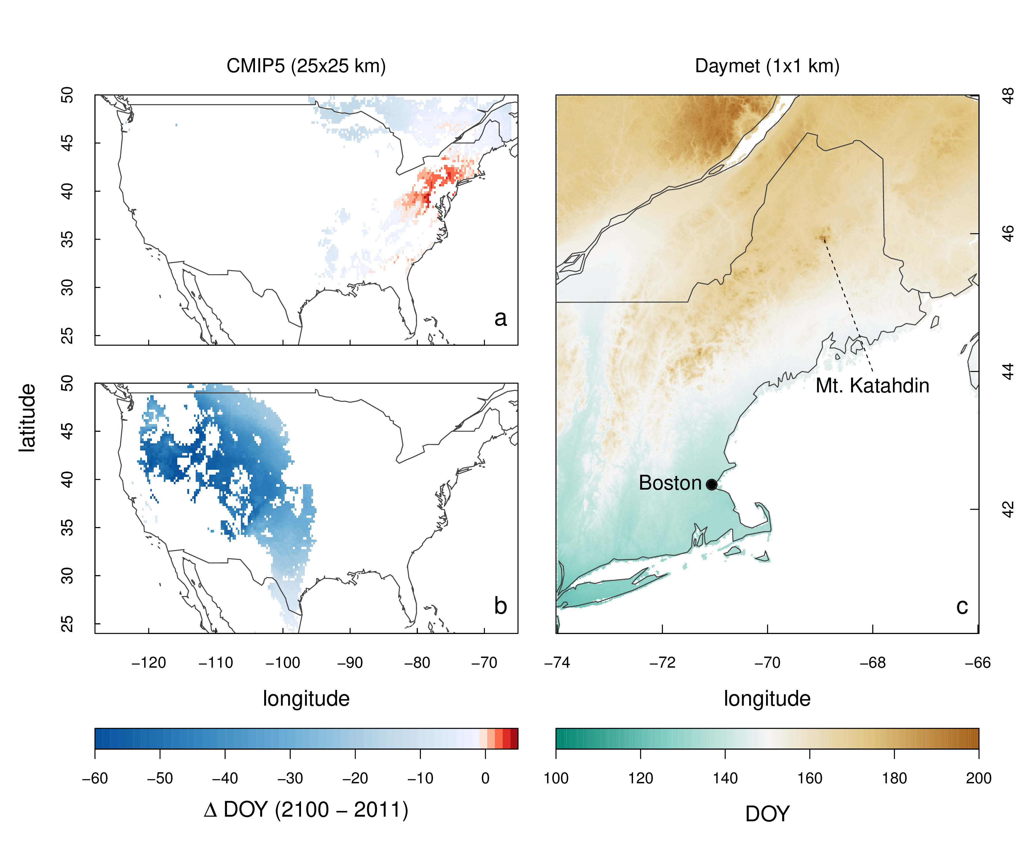
Figure 4.1: spatial scaling