3 Material and Methods

3.1 The phenor R package

The phenor R package assimilates four important phenological records of either observational, near-surface and satellite remote sensing based records across a variety of ecosystem and plant functional types. The phenor R package combines data from near-surface remote sensing through the PhenoCam network using phenocamr and daymetr R packages into a phenology modelling framework which covers data preparation, model optimization and model visualization and consists of a number of key functions. In addition, data from the USA National Phenology Network (USA-NPN), the Pan European Phenology Project (PEP725) and the MODIS land surface phenology product (MCD12Q2) can be ingested. In the interest of brevity both phenocamr, daymetr R packages and the PhenoCam source data are described in Appendix S1.

The format_phenocam() phenor function combines phenophases, downloaded and generated by the phenocamr R package, with the climate data downloaded using the daymetr R package. The function requires the location (path) of the generated phenophase output files, together with parameters specifying the phenophase (direction = rising; with rising for spring or falling for autumn) and the threshold value used (threshold = 25), the Gcc percentile to use (gcc_value = 90, Sonnentag et al. 2012) and the offset as a day-of-year value. The offset is the day-of-year in the previous year on which to start reporting climate data, running until this day in the subsequent year. The function returns model calibration/validation and driver data a nested list of data frames (df), used in subsequent model optimization (see description of optimize_parameters() and model_calibration() below).

df = format_phenocam( path = “/path/to/phenocamr/phenophases/”,
                           direction = “rising”,
                           gcc_value =  “gcc_90”,
               threshold = 25,
                           offset = 264)

Similarly, the format_pep725() function uses PEP725 observational data together with European E-OBS climate data (Haylock et al. 2008) to compile a consistent calibration/validation dataset for European observational records (e.g., Basler 2016). Data can be downloaded using the download_pep725() function. We provide similar functionality for the USA-NPN data. Data can be downloaded through the USA-NPN application programming interface using download_npn() and correctly formatted with format_npn(). Furthermore, the format_modis() function correctly formats a directory of MODIS MCD12Q2 land surface phenology data (i.e., phenophases, Zhang et al. 2003) as downloaded with the MODISTools R package (Tuck et al. 2014).

Spatially scaling of model results is facilitated through a number of functions. The format_daymet() function uses gridded pre-processed Daymet tiles to generate spatially explicit driver data (download_daymet_tiles() and daymet_tmean() functions of daymetr, Appendix S1). The format_eobs() function provides the same functionality for the E-OBS climate data. Yet another source of hindcast data is compiled using the format_berkeley_earth() function, which allows the user to subset 1x1 degree global historical climate data for any year since 1850 through the Berkeley Earth project (Rohde et al. 2012). Similarly, the format_cmip5() function formats 1/4th degree NASA Earth Exchange (NEX) global gridded Coupled Model Intercomparison Project (CMIP5) data of historical reanalysis and representative concentration pathway (RCP 4.5 and RCP8.5) projections. Unlike format_phenocam() or format_modis() no calibration/validation data is included in the gridded spatial data.

The resulting dataset of all formatting functions is a nested list with the following layout:

phenor_data_structure
    └─── doy (vector)
    └─── site (vector, NULL for spatial data)
    └─── location (matrix, latitude and longitude by row)
    └─── ltm (vector, value: degrees C)
    └─── Ti (matrix, columns: years, rows: doy, value: degrees C)
    └─── Tmaxi (matrix, columns: years, rows: doy, value: degrees C)
    └─── Tmini (matrix, columns: years, rows: doy, value: degrees C)
    └─── Li (matrix, columns: years, rows: doy, value: hours/day)
    └─── VPDi (matrix, columns: years, rows: doy, value: Pa)
    └─── Pi (matrix, columns: years, rows: doy, value: mm/day)
    └─── transition_dates (vector, NULL for spatial data)
    └─── georeferencing (NULL for PhenoCam, MODIS, USA-NPN or PEP725 data)
        └─── size (size of the spatial data)
        └─── extent (extent of the spatial data)
        └─── projection (projection of the spatial data)

Within the phenor data structure the top level is a particular site. For each site critical parameters such as the day-of-year range (doy, as specified by the offset), the geographic location (or georeferencing), and matrices holding, minimum temperature (Tmini), maximum temperature (Tmaxi) and mean daily temperature (Ti), precipitation (Pi), vapour pressure deficit (VPDi), daylength in hours (Li), and calibration/validation transition date (transition_dates) data are provided. Matrices are organized with columns representing a given year, and rows representing a given day-of-year. Other data are represented as vectors matching the number of columns present in the climate data matrices. Where necessary, data is truncated to match the available climate data. When certain data sources are missing the content of a field is set to NULL.

The optimize_parameters() function in the package allows for the easy optimization of model parameters. This function uses two common optimizers, GenSA (Xiang et al. 2013) and rgenoud (Mebane & Sekhon 2011). The GenSA algorithm combines both the Boltzmann machine and faster Cauchy machine simulated annealing approaches for fast optimizations (Tsallis & Stariolo 1995), while the genoud routine combines an evolutionary algorithm with a derivative based (quasi-Newton) method to solve difficult optimization problems (Mebane & Sekhon 2011). To optimize a calibration/validation dataset (df) one specifies a particular model (e.g., the Thermal Time model, TT), a defined optimizer (e.g., GenSA), an objective function such the root mean squared error (RMSE) and upper-lower parameter limits as well as parameter starting values when required. Additional control parameters, such as the maximum number or iterations (e.g., max.call), can be provided using a list of options to the control parameter. An example function call to optimize a the TT model is provided below.

optimal_par = optimize_parameters( par = NULL,
                    data = df,
                    cost = rmse,
                    model = “TT”,
                    method = “GenSA”,
                    lower = c(1,-5,0),
                                    upper = c(365,10,2000),
                    control = list(max.call = 40000))

Final predicted values for the optimized parameters can be retrieved by running the estimate_phenology() function with the optimized parameters.

results = estimate_phenology(par = optimal_par$par,
                    data = df,
                    model = “TT”)

The output will automatically be formatted as a map of phenology dates or a vector, depending on the input data class. However, running models across all grid cells of spatial data would provide a naively broad representation of land surface phenology. For example, only a small subset of the US is dominated by any particular plant functional type (PFT), such as deciduous broadleaf forests. In order to better differentiate between different dominant PFT we include a function land_cover_density() which calculates the percentage coverage of a particular MODIS MCD12Q1 IGBP land cover class (Friedl et al. 2010) within a given raster cell for a given location (i.e., CMIP5 data, see Figure 4.1).

A wrapper function, model_calibration(), is provided for both the optimize_parameters() and estimate_phenology() functions which integrates the previously described steps providing both summary statistics (RMSE and AICc) and a plot (Figure 3.1 ) of the model fit. Likewise, the model_comparison() function serves as a wrapper for multi-model parameter optimization runs. For a visual comparison limited to two model runs we provide an arrow plot function, arrow_plot(), displaying directional changes in the modelled values between the model outputs (Figure 3.2 ).

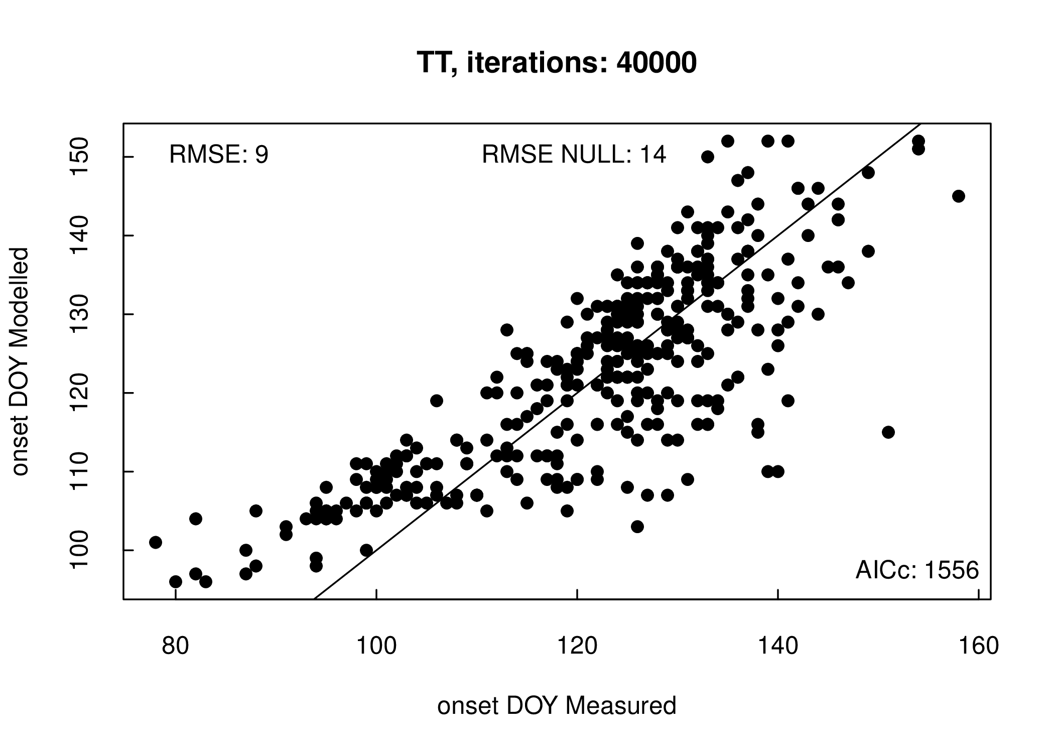
Figure 3.1: Model calibration output

Figure 3.2: Arrow plot

3.2 A worked example: a quick model comparison

As a worked example we partially recreate the spring phenology model comparison by Basler (2016) using PhenoCam data. However, we note that a similar exercise could be executed with any of the other phenology data sources available through phenor. The model structures included in this worked example can be described by the three broad categories: (1) as simple linear regression to spring temperature (2) models explaining ecodormancy release only, (3) models explaining the release of endo- and ecodormancy. A reference NULL model assumes a fixed mean date of leaf unfolding.

A total of 22 phenology models are included in the package (table 1). These include 20 spring phenology models including precipitation driven models, one fall senescence chilling degree day model and one grassland pollen release model. In our worked example of the phenor R package we will focus only on the 20 spring phenology models. A full list of the model structures and parameter ranges for the models are provided in Table 2 of Appendix S2 and included in the phenor library.

Table 1. Adapted from Basler (2016, Table 1). Overview of the phenological models for leaf unfolding and leaf senescence, and pollen release included in this study. The models are grouped by implemented processes and drivers: chilling temperatures (C), forcing temperatures (F), photoperiod (P), precipitation (R) and vapour pressure deficit (V). Function names in round brackets while full model structures are listed in Appendix S2 Table 1.

Model Name	Drivers	# of parameters	References
NULL	-	1	mean date of leaf unfolding
LIN	F	2	linear regression against spring temperatures
Thermal Time^a (TT, TTs)	F	3(4)	(De Reaumur 1735; Wang 1960; Cannell et al. 1983; Hänninen 1990; Hunter & Lechowicz 1992; Kramer 1994; Leinonen et al. 1997; Chuine et al. 1999)
Chilling Degree Day (CDD)	C	3	(Jeong & Medvigy 2014)
Photothermal-time^a (PTT, PTTs)	PF	3(4)	(Masle et al. 1989; Črepinšek et al. 2006)
M1^a (M1s)	PF	4(5)	(Blümel & Chmielewski 2012)
Alternating (AT)	CF	5	(Cannell et al. 1983; Murray et al. 1989)
Sequential^b (SQ, SQb)	CF	8	(Hänninen 1990; Kramer 1994)
Parallel (PA, PAb)	CF	9	(Landsberg 1974; Hänninen 1990; Kramer 1994)
Unified (UN)	CF	9	(Chuine 2000)
Sequential M1^b (SM1, SM1b)	CPF	9	Combination with the M1 model
Parallel M1^b (PM1, PM1b)	CPF	10	Combination with the M1 model
Unified M1 (UM1)	CPF	10	Combination with the M1 model
Growing Season Index^c (SGSI, AGSI)	FPV	7	(Xin et al. 2015)
Grassland Pollen model (GRP)	FR	5	(García-Mozo et al. 2009)

^a also calibrated using a sigmoid temperature response (Hänninen 1990; Kramer 1994). adding one parameter. ^b also calibrated using a bell-shaped chilling response (Chuine 2000). ^c calibrated using a cummulative response rather than the rolling mean.

For this study we combined spring phenology dates based on PhenoCam 3-day summary data from the standardized PhenoCam Dataset (Richardson et al. 2017) with Daymet data (Thornton et al. 2017) for three common PFTs, deciduous broadleaf forests, evergreen needleleaf forest and grasslands. A total of 102 sites and 508 site years were included in our calibration/validation dataset, of which 63 were deciduous broadleaf forest sites (358 site years), 18 were evergreen needleleaf forest sites (63 site years) and 21 were grasslands (88 site years). Deciduous broadleaf sites which are moisture limited, and all sites outside Daymet coverage, were excluded from our analysis. The final selected sites span a large geographic area ranging from New Mexico to Southern Alaska, and Maine to California (Figure 3.3).

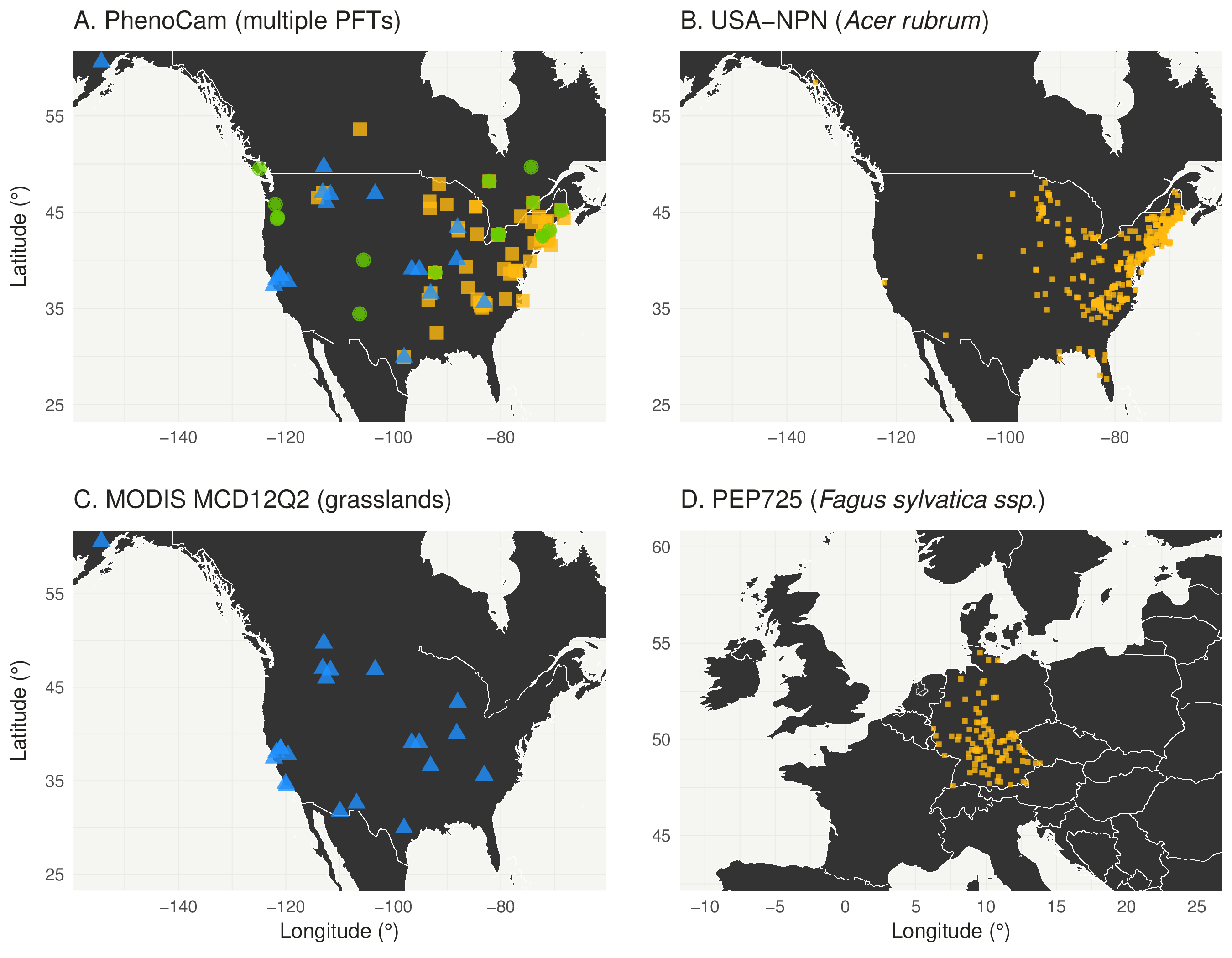
Figure 3.3: Site locations

We acknowledge that phenological development as measured using PhenoCam data represent different physiological processes for different PFTs. For example, the phenology of deciduous forests or grasslands is closely linked to the development of new leaf tissues (Keenan et al. 2014; Hufkens et al. 2016) where evergreen forest phenology is determined by dehardening of existing needles at the end of the winter season. Thus, optimized model parameters and their interpretation are specific to each PFT.

For all PFTs, model optimization were executed using the default generalized simulated annealing (GenSA) package minimizing the RMSE between the greenness rising PhenoCam phenophase estimations and model predictions (see Appendix S1). The optimizer was run for 40 000 iterations with a starting temperature of 10 000. To determine the influence of locations at the margin of the forest biome on model optimizations a subset of sites centrally located within the deciduous forest biome was created (Melaas et al. 2016, Appendix S2 Table 2). This subset was optimized separately and compared to results for the complete deciduous broadleaf dataset. We assess proper convergence of the optimized parameters by initializing the optimizer using 12 random sets of parameters. We report mean and standard deviations of the RMSE between observations and predictions on the optimized parameter values for all PFTs and the subset generated for deciduous forest sites. We compare model performance with a log transformed ANOVA, combined with a post-hoc Tukey HSD test. Model errors are evaluated for normality using a Shapiro-Wilk test.

For illustrative purposes we produce overview maps (Figure 4.1) of spatial patterns both in hindcast and forecast mode. In hindcast mode we use 1x1 km Daymet gridded data across New England, while we present the difference in predicted spring phenology (ΔDOY) between years 2100 and 2011 for forecast CMIP5 IPSL-CM5A-MR (Mid-Resolution Institut Pierre Simon Laplace Climate Model 5) model runs, across the contiguous US. The Thermal Time (TT) and Accumulated Growing Season Index models were optimized for deciduous broadleaf and grassland PhenoCam data, respectively. For forecast data only pixels dominated by their particular PFT are displayed, limiting a naively broad interpretation of the results.

Our comparison of 20 spring phenology models across three PFT showed that most models were significantly different from the NULL model, with the exception of the SGSI model in the evergreen PFT (post-hoc Tukey HSD test, p < 0.001, Figure 3.4). The model performance of the centrally located deciduous broadleaf sites was marginally greater (RMSE: ~7.6±0.7 days) compared to the complete deciduous broadleaf dataset (RMSE: ~7.9±1.2 days). This difference between the full deciduous broadleaf forest dataset and those more centrally within the biome suggests an influence of geographic location on model error.

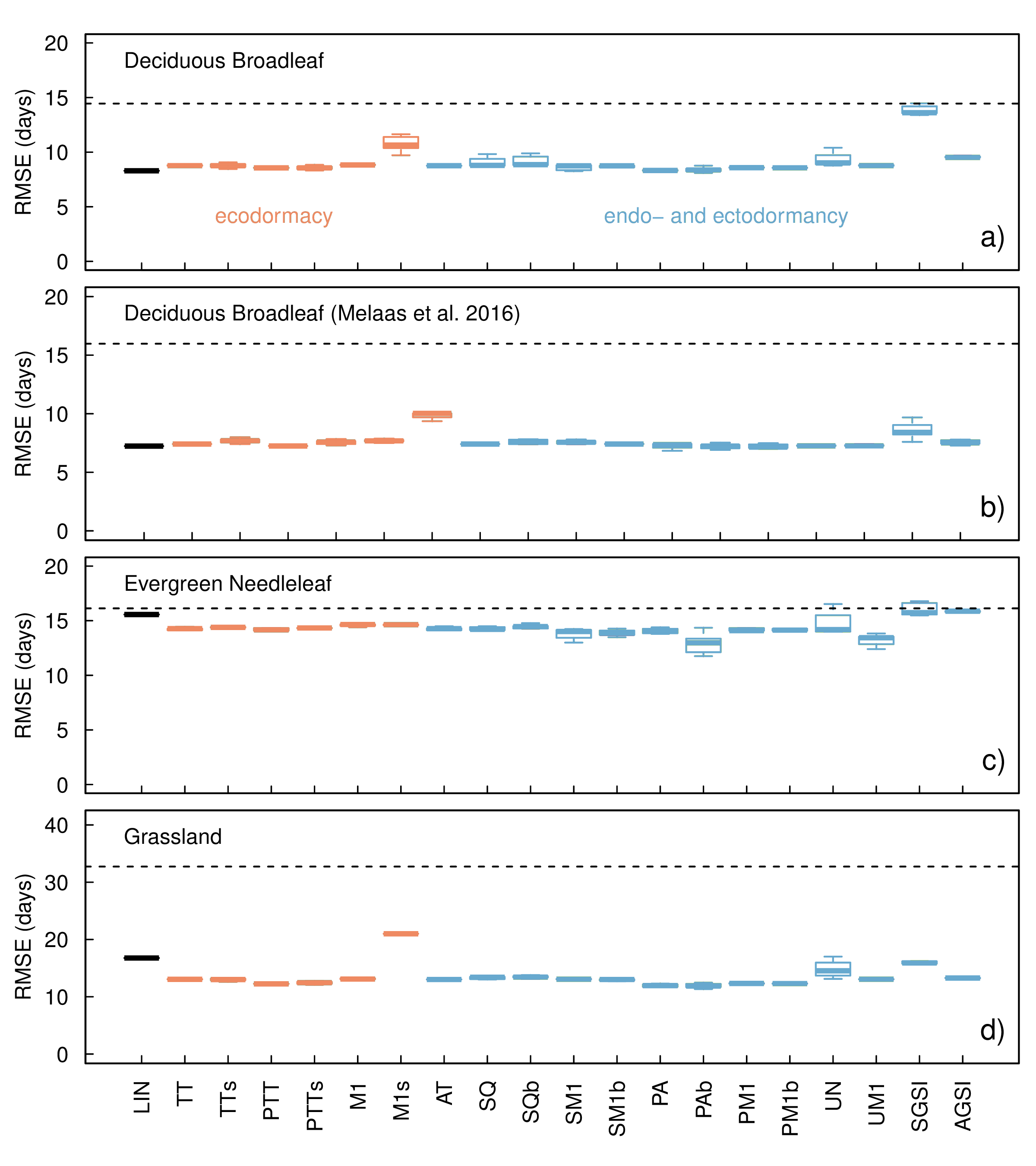
Figure 3.4: model comparison

The influence of different model structures on individual values was visualized using the arrow plot (Figure 3.2) between two model runs. When visually comparing the Thermal Time (TT) and the Photothermal Time (PTT) models small changes are noted (3.2). Both models accumulate growing degree days where the PTT model adds a photoperiod component to the original TT model. In the PTT model leaf unfolding is therefore in part dependent on a daylength requirement in addition to thermal forcing. In our example, the addition of a daylength requirement shifts model results for early and late developing plants toward earlier leaf out dates, while at the same time shifting mid season developing plants toward later leaf out dates. Despite these changes overall model accuracy remains the same.

In particular, comparing model performance across the 20 spring phenology models and all the three PFT showed that all models were significantly different from the NULL model, except for the SGSI model for the evergreen PFT (post-hoc Tukey HSD test, p < 0.001, Figure 4). We also note that the NULL model for the grassland PFT performed worse compared to either evergreen or deciduous forest PFT (Figure 4d). For grasslands the RMSE of the NULL model equals 32.7 days compared to only 14.5 and 16.1 days for the deciduous and evergreen forest sites respectively. Excluding the NULL model, model RMSE varied greatly among PFTs. For deciduous broadleaf sites an average RMSE of ~9.1 ± 1.2 days was observed (Figure 4a). For the evergreen needleleaf forest and the grassland sites the RMSE values almost doubled (~14.4 ± 0.8 days and ~13.6 ± 2 days respectively, Figure 4c-d). A separate model optimization on centrally located deciduous broadleaf sites resulted in a RMSE ~7.6 ± 0.7 days (Figure 4b). Limiting the deciduous broadleaf sites to locations to those centrally located within the biome point to a marginally higher RMSE of ~7.9 ± 1.2 days. Differences between the full deciduous broadleaf forest dataset and those more centrally within the biome allude to the influence of geographic location on model error. Although our analysis quickly and easily reproduced a limited version of previous work by Basler (2016), only including a subset of the models discussed and omitting extensive cross-validation therein, our study extends this work in other ways. Mainly, we increased the geographic range, covering boreal, temperate and subtropical regions, and included three plant functional types. However, even with this greater range in latitude and the continental scale of the study, as well as three plant functional types, does not change previous findings.

Variability between in RMSE between the PFT can largely be explained by differences in phenological processes. Grassland phenology is largely determined by both temperature and plant available water. Yet, two grassland spring phenology models included in phenor which account for water stress through VPD (SGSI, AGSI; Xin et al. 2015) do not perform significantly better than other described models. Heterogeneity, between grassland locations might explain this lack of performance. However, an in depth analysis is outside the scope of this manuscript. Evergreen forest phenology as observed by PhenoCams is not determined by developing leaves but by dehardening of existing needles. Estimates of evergreen phenology therefore might benefit from a model structure focussed on the dehardenning process (Hänninen & Kramer 2007) not yet included in the described models.